Mall-Scale Water Feature Design
In this lab a nozzle that was capable of shooting beams of water between specified distances was designed. To accomplish this task, an in depth understanding of pump characteristics and internal flow was needed. Experiments were conducted which allowed us to measure the pressure and volumetric flow of the pump at different operating speeds. These experiments provided us with the values that were needed to graph our pump curves. To find the operating point of our pump, the point at which our system curve intersected our pump curve needed to be found. Using a variety of nozzle diameters, the optimal volumetric flows for our system were calculated. The water streams were modeled using the kinematic equations and thus the operating settings for our system were determined.
A nozzle was modeled on SolidWorks and was tested to see if our calculations were correct. Based on the results of this experiment, it was determined that there was a calculation error with the angle of the nozzle which caused the setup to fail. To confirm this theory, the angle of the nozzle was decreased and the water stream successfully made it into the tank.
Once the settings of the pump as well as the details of our setup were determined, an economic analysis was performed to determine costs of operating this pump as well as the costs of the materials. Using probabilistic economic analysis, it was determined that using a plastic nozzle, as opposed to a stainless steel one, produced a lower annual cost, even though it would need to be replaced more often.
Introduction
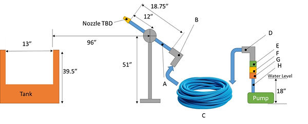
Many hotels and malls include water features that use massive pumps to shoot beams of water between specified distances. Being able to complete such a feat requires great understanding of pump characteristics and internal flow. The purpose of this lab was to perform the necessary calculations to create a shopping mall scale water feature system. The system would need to pump water from a tank and push the water through a variety of fittings and pipes which would all produce frictional losses. At the end of the system a nozzle was designed which needed to be capable of shooting the water over a specified distance and allow the water to collect in a tank. A diagram of the system configuration can be found in Figure 1.
Figure 1. Required system configuration.
The system starts at the pump on the right-hand side of Figure 1. The water then goes through a piece of poly tubing and a hose barb which expands the diameter of the tube from 1.9cm to 2.54cm. Then the water does through another reducer which brings the diameter down to 1.52cm and allows it to fit into the pipe section at E. The water then goes through a 90-degree elbow and goes into a 15.24m length of PEX tubing. The end of this tubing is connected to another 90-degree elbow and is connected to a .48m PVC pipe with a flange on the end. It is by this flange that the nozzle is connected to the rest of the system.
In this experiment, a nozzle was designed and pump speed, as well as the angle of the tube, which would allow us to convey a jet of water from the point of discharge to a tank approximately 96 inches away while operating 40 hours per week, 52 weeks per year were found. Secondly, the cost to own and operate this system was minimized by optimizing pump power and associated material costs.
Conceptual Design
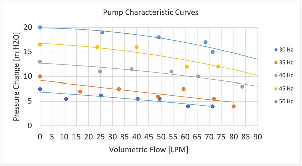
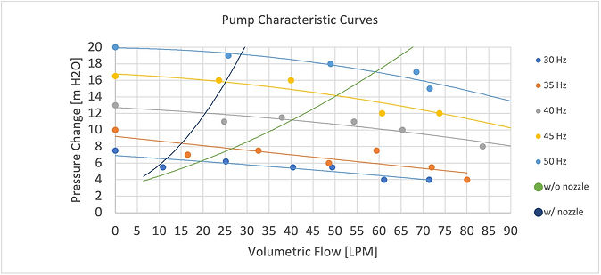
In a previous experiment, we created a setup in order to obtain the characteristics of the pump that we would be using in our water feature. Our experimental setup included a centrifugal pump with a variable frequency drive that allowed us to change the speed of the pump. Pressure gauges were added to the inlet of the pump as well as the outlet of the pump. The pressure difference between these two pressure gauges allowed us to calculate how much pressure was being added to the fluid by the pump. In order to generate pressure in the pump, a valve was attached to the pump outlet. By slowly constricting the valve, we calculated a range of pressures that our pump could generate. Finally, we used a stopper at the bottom of our tank to measure the volumetric flow of the pump. All of these values allowed us to generate the pump curves shown in Figure 2.
Figure 2. A plot of the pump characteristic curves.
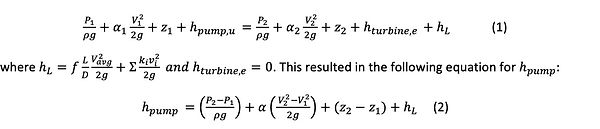
To find the operating point at which we could use the pump, we had to model the system to account for of the frictional losses that would occur from the various fittings and pipes. In order to do this, we will use the following internal flow equation:
We are able to determine the as a function of the volumetric flow rate, also known as the system curve. We calculated two curves: one with the nozzle and the other without the nozzle. We did this so that we could verify that the nozzle was needed for our system to meet the distance criteria. The pump in our water feature will operate at the point where the system curves and the pump characteristic curves intersect. Figure 3, shows the addition of these curves on Figure 2.
Figure 3. A plot of the system curves with the pump characteristic curves.
To graph the system curve for the nozzle, we had to know what our nozzle diameter would be this step was added after we had already determined our desired nozzle exit velocity. We knew the speed that we could get at the flange where the nozzle would be attached. Because we are looking to optimize power, I knew that I’d be looking for a volumetric flow that was on the lower end of our graph. Keeping this in mind, we made an estimate of the speed at the flange, and used this value to calculate a variety of speeds we could expect at the end of the nozzle based on different nozzle diameters.
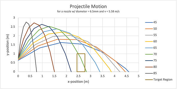
To determine which nozzle velocity to choose, we used the following kinematic equations to model the motion of the water beams:
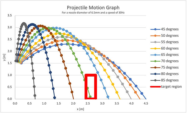
It was at this step we also needed to figure out which angles would be optimal for our design. We plotted the projectile motion curves for a variety of different speeds. Once we found what speeds worked out, we plugged the nozzle diameters into the system curve equations to get a system curve with the nozzle. We adjusted the calculations to match the volumetric flow and speed where the system curve intersected the 30Hz pump curve. This was at approximately 11 LPM which resulted in a flange exit velocity of 1.45m/s. Based on the projectile motion graphs that resulted from our analysis, we settled on a nozzle with a diameter of 6.5mm. The outlet velocity with the 6.4mm diameter nozzle was 5.58 m/s. A plot of the water beam’s motion is shown in Figure 4.
Figure 4. A plot of the water beams at different angles for a 6.5mm nozzle.
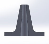
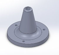
Using this diameter, we modeled a nozzle in SolidWorks. The cross-sectional and isometric views of the nozzle, as well as a dimensioned drawing, can be found in Figure 5.
Figure 5. A cross-sectional (top left), isometric view (top right), and dimensioned drawing (bottom) of the 6.5mm nozzle.


Experimental Validation & Results
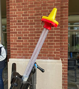
We set up the system described in Figure 1 with the tube at 70 degrees and the pump set at 30Hz. The nozzle did not work successfully and did not go as far as we had calculated in our conceptual design. We measured that the beam of water shot a distance of around 7’. In order to find out what we did wrong, we tried manipulating the angle of the tube and found that our setup worked at an angle of 60 degrees.
After the lab experiment, it was evident that I had made a couple calculation errors. When taking a closer look at Figure 4, it appears that the initial height of the water beams is lower than the height of the tank. According to Figure 1, the height of the tank is 39.5” and the height of the stand is 51”. This error was corrected and resulted in the projectile graph in Figure 6.
Figure 6. A plot of the adjusted projectile motion curves.
However, even after adjusting the projectile motion graphs, it seemed like my setup still wouldn’t work. According to my calculations, shooting a beam of water at 60 degrees would’ve made my beam of water overshoot the tank by at least half a meter. This error seems to be because of some assumptions I’ve made for the projectile motion. Because the beam of water is a continuous mass and not a point mass, the kinematic equations can’t perfectly predict the motion of the water. Additionally, I’ve neglected air resistance in my calculations which would shift the curves slightly to the left.
Economic Analysis
In our project requirements, it is stated that this system is to be running 40 hours per week, 52 weeks per year. Therefore, it makes sense that we try and take any steps to minimize costs. In terms of the pump’s operation, we’ve already taken the steps to lower the amount of power used by the pump because we are running at 30 Hz. However, we can minimize the costs further by choosing what material the nozzle is made out of. In Appendix Table 1, is a table with the economic parameters for the nozzle material costs and lifetime, electricity costs and lifetime, and the discount rate. However, because these values are given as ranges, we will be using probabilistic analysis. By doing this type of analysis, we can use both the worst- and best-case scenarios to inform our economic decisions.
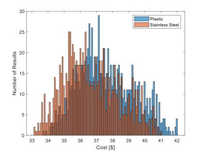
Since all the economic inputs in the economic analysis can vary overtime, they can be treated as a probabilistic function. For example, since it is known that the cost of plastic varies from $0.02-$0.05/cm3 with a mean of $0.03/cm3, we know that the distribution would be triangular with one end of the triangle at $0.02, the other at $0.05, and the tip of the triangle at $0.03. To perform the probabilistic analysis, probability density functions were created using these triangular distributions which utilized the high, low, and mean values provided in the table. From these probability density functions, cost predictions were generated randomly resulting in a distribution for the costs of both the plastic and stainless-steel nozzles. These cost predictions were performed in MATLAB.
The result of our analysis allows us to state with 95% confidence that the plastic nozzle will cost $37.55 ± 3.49 every year and the stainless-steel nozzle will cost $36.66 ± 3.46 every year. Thus, it would be in our best interest to use a plastic nozzle. A histogram of the cost distributions is shown in Figure 7.
Figure 7. EAC cost distributions for a plastic or stainless-steel nozzle.
Final Reccomendations and Conclusions
The purpose of this experiment was to create a water feature that would be capable of shooting a beam of water across a specified distance. According to our calculations, in order to achieve the lab criteria, a system with a pump speed of 30 Hz, a nozzle diameter of 6.5mm, and angle of 70 degrees was required. After conducting the experiment, it was found that our launch angle was off by ten degrees and the system needed to be shifted to 60 degrees in order to work properly. However, even after recalculating the launch angle, our projectile motion was still off. It was assumed that because the beam of water is a continuous mass and not a point mass, the kinematic equations can’t perfectly predict the motion of the water. Additionally, air resistance was neglected in the calculations which would shift the curves slightly to the left. Finally, an economic analysis was performed to find an annual cost for a plastic and a stainless-steel model. Probabilistic analysis was used in order to produce a range of cost values for each nozzle. The result of our analysis allowed us to state with 95% confidence that the plastic nozzle will cost $37.55 ± 3.49 every year and the stainless-steel nozzle will cost $36.66 ± 3.46 every year.